Spectragryph
- optical spectroscopy software -

Functions of the Process ribbon => Click onto a button for descriptions

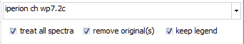
General options for processing functions: For most processing functions, you will get a specific window for setting parameters and options. Some of those options are identical for most of the functions: - At the top, there is a dropdown selector containing the current spectra list. Here you can select the spectrum to be processed (if only one spectrum gets treated). If a preview is available, the spectrum is selected here. - if the "treat all spectra" option is checked, all spectra will get processed and attached as new spectra at the end of the spectrum list. Otherwise, only the currently selected spectrum gets processed. - With the "remove all" option checked, the original spectra will be removed and only the processed spectra/ spectrum remain(s) . - The "keep legend" option leaves the original legend text unchanged. If unchecked, a function-specific text part will be added to the legend text.

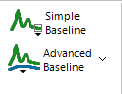
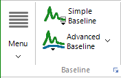
Simple Baseline subtraction For offset-correcting of straight baselines that deviate from zero. After clicking the button, use the left mouse button in the plot to select the x axis range which should be set to zero. The mean value of y values in the selected region will be subtracted from the spectrum as a constant value. It is done for all spectra at once. Advanced Baseline subtraction For cases, where a simple offset baseline correction doesn't work, this menu function gives advanced possibilities with three different baseline creation algorithms available. Select the baseline algorithm and its parameters from the button's dropdown menu entry "Baseline Options". A baseline preview will be shown and updated for the selected spectrum, based on current settings. . 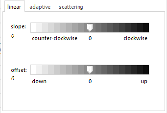For the linear baseline, you can adapt these parameters: - slope: changes the angle of the straight baseline (0 is horizontal). - offset: creates a vertical shift. 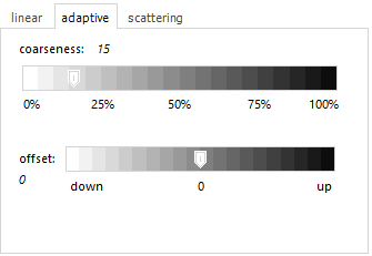The adaptive algorithm creates a baseline that snugly fits to the bottom of spectra. The intention is to remove broad underlying features (like fluorescence background in Raman spectra), while keeping actual peaks. A smaller coarseness value creates a tighter fit, with Offset you can have a vertical shifting of the baseline. This algorithm is a single-run, no-fitting, non-iterating algorithm. It creates a baseline by applying a 0% percentile smoothing, followed by a moving-average smoothing, with the same interval size for both steps (coarseness translates to interval size). 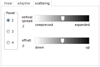The "scattering" algorithm is intended for absorbance spectra of scattering solutions, which have a continuously falling baseline towards long wavelengths. Depending on the size of scattering centers/ particles, the scattering intensity corresponds to 2nd to 4th power of the wavelength. Additionally, the vertical spread and offset can be adapted. On clicking "Apply", the created baselines will be subtracted from the original spectra. With "individual baseline" selected, a separate baseline is created for each individual spectrum (the default behaviour). In case of "create baseline spectrum" is checked, the used baselines will be added as actual spectra to the list of spectra. Clicking the main button will execute baseline subtraction on all spectra, based on the currently defined parameters (but only if "treat all spectra" is selected).

<jump back to top>

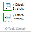
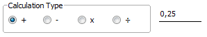
x Offset/ Stretch This applies a constant value with the selected calculation type to the spectrum's x axis values. Depending on the selected calculation type, you can shift spectra to left/right (addition (+), subtraction (-)), stretch (multiplication (x)) and compress (division (÷)) along the x axis. Hint: Please use this function only if you really know what you are doing, since it modifies the spectra in a rather unusual manner. y Offset/ Stretch This applies a constant value with the selected calculation type to the spectrum's y values. Depending on the selected calculation type, you can shift spectra up (addition (+)) and down (subtraction (-)), stretch (multiplication (x)) and compress (division (÷)) along the y axis. The latter two functions are often used for normalizing spectra manually. As an alternative, you can do both, x and y offsetting and stretching interactively to individual spectra by using the Scale/Shift function from the Plot/Views ribbon.

<jump back to top>

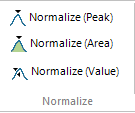
Normalization With normalization, you bring the y scale of spectra into a similar range, for comparing spectrum shapes, original y value relations between spectra get lost. Several methods are available: Normalize (Peak) All Spectra are scaled such that their highest peak in the currently visible x axis range is set to a value of 1. Select the desired x range before using the function. It always applies to all loaded spectra and acts on the spectra, no new spectra will be created. Normalize (Area) All Spectra are scaled such that the area under curve within the selected x axis range has the same value. After clicking the button, it waits for you selecting the desired x range with the left mouse button. It always applies to all loaded spectra and acts on the current spectra, no new spectra will be created. Normalize (Value) This function will scale spectra, so that they have all a certain value at a certain x position. Here all the usual options are available, like treat one or all spectra, remove original, keep legend.

<jump back to top>

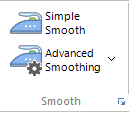
Simple Smooth For quickly smoothing all spectra at once, no options available, smoothed spectra added to the end of spectra list. As smoothing algorithm, a 3rd order Savitsky-Golay smoothing is used, with an interval size depending on each spectrum's actual data point step width. Advanced Smoothing For better control of smoothing behaviour, with a choice of smoothing algorithm and smoothing parameters. Four algorithms are currently available. Select the smoothing algorithm and its parameters from the button's dropdown menu entry "Smoothing Options". A preview of the smoothed spectrum will be shown and updated for the selected spectrum, based on current settings. 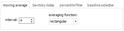moving average smoothes by calculating an average value for every data point from all neighboring data points within the selected interval size. A rectangular or triangular shape can be choosen as weighting function for averaging. With the triangular shape, more distant data points are down-weighted. 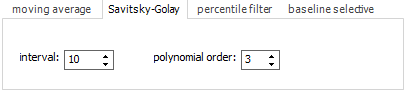Savitsky-Golay smoothes by calculating a least-squares polynomial interpolation value for every data point from all neighboring data points within the selected interval size. The interval size and the polynomial order can be choosen. 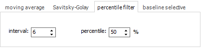Percentile filter smoothes by identifying the selected percentile for the neihgbouring data points within the interval size for every data point. A lower or upper envelope spectrum results on choosing the 0% or 100% percentile. 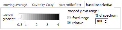Baseline-selective smoothing is a special algorithm working best on spectra with baseline areas near to zero, like Raman spectra after baseline subtraction and some UV/VIS and FTIR spectra. It is based on Savitsky-Golay smoothing with increasing smoothing interval size towards the baseline area at low y values. The gradient of this increase can be changed with the slider and the mapped y axis range can be defined in two ways. Just give it a try on your spectra... The benefit is: have less noise in baseline area without significantly changing actual peaks! On clicking "Apply", the defined smoothing algorithm will be applied on spectra.. Clicking the main button will execute advanced smoothing on all spectra, based on the currently defined parameters (but only if "treat all spectra" is selected).

<jump back to top>

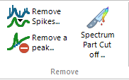
Remove Spikes With Silicon-based CCD detectors, artifacts from cosmic radiation are increasing with longer exposure times (several seconds). These are called cosmic spikes. This function detects spikes and interpolates the spectrum in the range of the spike. All other spectral data points remain totally unchanged. Spectra without spikes remain also unchanged. As an option, you can define the maximum width for a found spike location (default is 5 pixels). Any found, wider spike artifact is not removed, to make sure not to change spectral features. Use a smaller value for spectra with poor resolution, in order to prevent erroneous removal of narrow spectral peaks. Another options is "backward removal" which applies the same algorithm from right to left, thus occasionally finding some undetected spikes from a first run. Hint: you will find a myriad of cosmic spike removal algorithms in literature, many of which are rather complicated. I devised this simple algorithm for my own use around year 2001-2002, it was already part of the previous Spekwin32 software for many years. The algorithm is based on the very different shape of a spike artifact compared to a spectral peak in the spectrum's 1st derivative. Based on this differentiation, the assigned spike area gets interpolated by a moving average. For a long time, I couldn't find something comparable in literature. It seems, this finally changed in 2018... Remove a peak This function exactly does what its name says. Just enter the peak location and its FWHM and the spectrum gets interpolated in that area. Hint: There are only few uses, where making a measured peak go away is considered a proper task. Handle with care! Spectrum Part Cut off For cutting away a part of the spectrum from one or both sides (start and end). Enter the new start and end values for the remaining range manually, or else interactively move the two vertical cursors shown together with the function's window. After applying the new boundaries with Apply, the window will stay open to allow more changes. When finished, click the Close button.

<jump back to top>

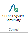
Correct System Sensitivity For correcting the wavelength-dependent system sensitivity (mainly introduced by fibers, gratings and detectors) of emission spectrometers (fluorescence, Raman, radiometry...). Sensitivity correction yields "true spectra" as output. Load the correction curve with the Load correction Curve button (any file format accepted, data should consist of sensitivity against wavelength). Spectral data will be divided by the loaded correction curve, which persists for the current session.

<jump back to top>

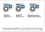
Chemometric preprocessing For preparing spectra for chemometric analysis, a number of processing steps are often used, like file conversion, baseline removal, normalization, smoothing, derivatives and so on. These three functions are often used as a data pretreatment especially on NIR spectra before actual chemometric analysis, in order to remove time-dependent drift that is irrelevant to actual sample characteristics, but would interfere with analysis. Recommended reads for in-depth explanation of such algorithms can be found here, here and here. SNV (standard normal variates) is often used on spectra where baseline and pathlength changes cause differences between otherwise identical spectra. It works by normalizing the averages of whole spectra. MSC (multiplicative scatter correction) has proven to be effective in minimizing baseline offsets and multiplicative effect. It is achieved by regressing a measured spectrum against a reference spectrum and then correcting the measured spectrum using the slope and intercept of this linear fit. You can either load a reference spectrum or use an average of the whole data as reference. Detrending is performed through subtraction of polynomial fit of baseline from the original spectrum to remove tilted baseline variation, usually found in NIR reflectance spectra of powdered samples. The order of the used polynomial can be selected.

<jump back to top>