Spectragryph
- optical spectroscopy software -

Functions of the Analyze ribbon => Click onto a button for descriptions

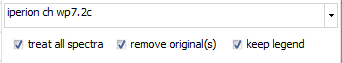
General options: For all functions, you will get a specific window for setting parameters and options. You will find the top spectrum selector with all Analyze functions, while the checkboxes only exist with "Gaussian Deconvolution": - At the top, there is a dropdown selector containing the current spectra list. Here you can select the spectrum top be analyzed (if only one spectrum gets treated). If a preview is available, the spectrum is selected here. - if the "treat all spectra" option is checked, all spectra will get processed and attached as new spectra at the end of the spectrum list. Otherwise, only the currently selected spectrum gets processed. - With the "remove all" option checked, the original spectra will be removed and only the processed spectra/ spectrum remain(s). - The "keep legend" option leaves the original legend text unchanged. If unchecked, a function-specific text part will be added to the legend text.

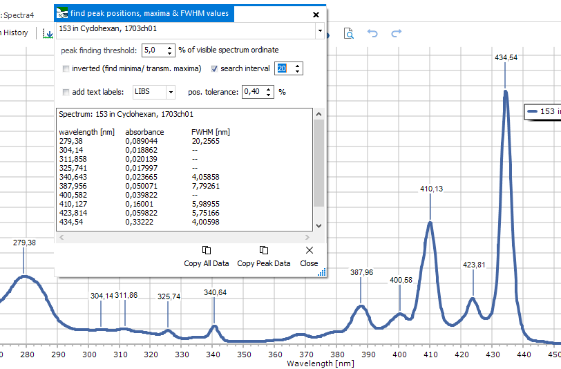Peaks & FWHM For the currently visible x axis range, a list of peak positions together with their FWHM values is created. A number of parameters can be set: peak finding threshold: sets the lower limit of the found peaks, just the same as it is done with the Peak labels function. search interval: a smaller value finds less prominent peaks, this parameter corresponds to the prominence parameter from the Peak labels function. inverted (find minima/ transm. maxima): will search for minima add text labels: to be used with the special label types, like LIBS, XRF, Gamma. It adds an additional column to the list with the respective position labels (atom names for LIBS and XRF, nucleids for Gamma). On the right, the position tolerance can be set, to ensure selection of only the proper assignments. Copy Peak Data: this button copies the list to the clipboard, to be pasted for further use into other software. Copy All Data: this button copies a concatenated peak list for all spectra to the clipboard, to be pasted for further use into other software.

<jump back to top>

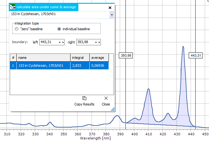
Integration For calculating the area under curve within a given x axis range. Enter the new start and end values for the integral range manually, or else interactively move the two vertical cursors shown together with the function's window. The results list shows a table of integral values for all spectra, together with an average value of the same area (just ignore that if you don't need). In the plot, the area under curve gets visualized for the currently selected spectrum in the upper spectrum selector. The area shape depends on the chosen integration type: - "zero" baseline : uses the x axis as a straight lower boundary for integration. This only makes sense for spectra with an existing baseline near zero. - individual baseline : uses a straight, but tilted line as lower boundary, that connects the start and end point of the integral area. Copy Results: this button copies the results list to the clipboard, to be pasted for further use into other software.

<jump back to top>

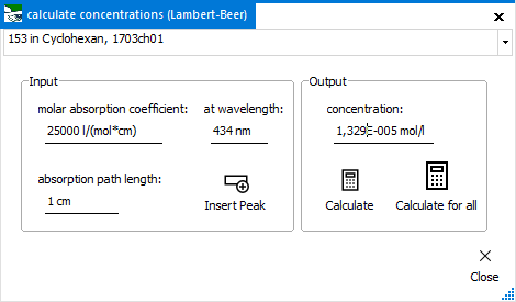
Concentration (from spectrum) To calculate the molar concentration for a certain spectrum from its absorbance spectrum. For this function, the molar absorption coefficient has to be known. The calculation is done via Lambert-Beer. All entered values apply only to the spectrum selected in the upper spectrum selector. After entry of values for molar absorption coefficient, wavelength and absorption path length, you can calculate the concentration with the Calculate button. The Calculate for all button does the same, but for all spectra at once (which makes sense for a concentration series of the same subtance, for example). Instead of manually entering the wavelength value, this field can be filled with the current spectrum's maximum position with the Insert Peak button.	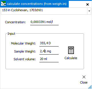Concentration (from weighing) To calculate the molar concentration for a certain spectrum from its molecular weight and solution creation. After entering the molecular weight, sample weight and solvent volume, calculate the molar concentration with the Calculate button. The same calculation is also possible from the Data tab within the Spectra Properties window, where you can also manually enter the concentration value.
The calculated concentration value gets saved together with the spectrum in the *.sgd file format. HINT: Only with a concentration value assigned, the switching of y axis type to molar extinction coeefficient or its logarithm gives a meaningful display!
<jump back to top>

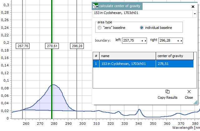Center of Gravity For calculating the center of gravity of a spectrum peak area within a given x axis range. Enter the new start and end values for the horizontal range manually, or else interactively move the two vertical cursors shown together with the function's window. The results list shows a table of center position values for all spectra. In the plot, the area under curve and the center of gravity (green vertical line) get visualized for the currently selected spectrum in the upper spectrum selector. The area shape depends on the chosen area type: - "zero" baseline : uses the x axis as a straight lower boundary for calculation. This only makes sense for spectra with an existing baseline near zero. - individual baseline : uses a straight, but tilted line as lower boundary, that connects the start and end point of the area. Copy Results: this button copies the results list to the clipboard, to be pasted for further use into other software.

<jump back to top>

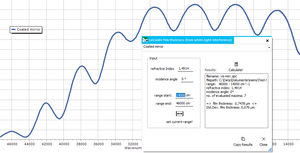Film Thickness From a white-light reflectance spectrum showing interference, the thickness of a single-layer thin film can be calculated. As input values, the refractive index of the film material is needed together with the incident angle of the reflected light (perpendicular illumination means an angle of 0°) The used wavelength/ wavenumbers range can be changed manually or by clicking the set current range button. Clicking the Calculate button fills the results output window with the calculation results. The results window contains the input data, the number of evaluated peaks and the calculated thickness together with a quality measure (standard devation). A StDev value higher than a few percent of the thickness value indicates an invalid result. While the calculation is done on the wavenumbers spectrum, it is no necessary to switch the display to wavenumbers before calculation. 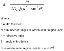The calculation is based on this equation. It only works for a single-layer thin film!

<jump back to top>

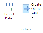
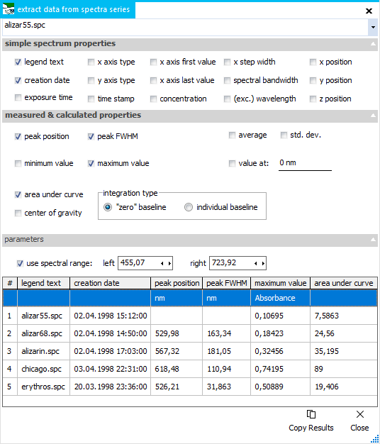
Extract Data This function creates a data table for a loaded spectra series, listing the values of selected parameters within a given x axis range. After clicking the Extreact Data button, select the x axis area with the left mouse (like zooming), then the window is shown. Change the start and end values for the integral range manually, or else interactively move the two vertical cursors in the plot. Calculated properties in the data table will be updated on the fly, when the spectral range gets changed. As ssecond row, the parameter's units are shown, if available. For each selected parameter, a new column will be created in the data table. There are parameters for simple spectrum properties that do not depend on the spectral range, like legend text (checked per default), creation date, time stamp, first and alst value and some more. Then there is a range of measured and calculated parameters, most of which are already known from functions elsewhere, like highest peak position and FWHM, minimum and maximum value, average and standard deviation, area under curve and center of gravity. Additionally, the y value at a defined position can be shown, which represents a spectral cross section of the spectrum series. With "use spectral range" unchecked, the calculated properties are taken from the whole spectral range. Copy Results: this button copies the data table to the clipboard, to be pasted for further use into other software. HINT: for a spectrum series with time stamps (like all spectra measured with Spectragryph from a connected spectrometer), you can easily create a time series with this function. Just select "time stamp" as parameter and use this later as x value.

<jump back to top>

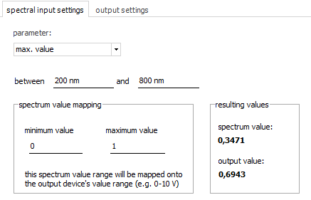
Create Output Value This function caculates a spectrum property (similar to the Colorize by property function) and sends it to a physical hardware as output device. The spectrum property's value range gets mapped to the value range of the output device, like a voltage or a colour, or whatever. Selecting another spectrum in the upper spectrum selector updates the sent output value. 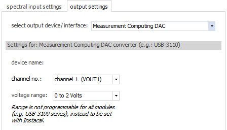As parameter, you can select: - y value (at a defined position) - minimum value (in a defined range) - maximum value (in a defined range) - average of y values (in a defined range) - standard deviation of y values (in a defined range) - area under curve (in a defined range) - peak position (in a defined range) - center of gravity (in a defined range) Currently, there is only one type of output device recognized: the range of DAC (digital analog converter) devices from Measurement Computing, like the USB-3110. You can define the channel number, as well as the actual voltage range from the dropdown selectors. HINT: The Create output value function is also available as post-procesing option for live spectra acquisition in the Acquire ribbon, therefore allowing to continuosly feed a physical representation of a spectrum property into another system.

<jump back to top>

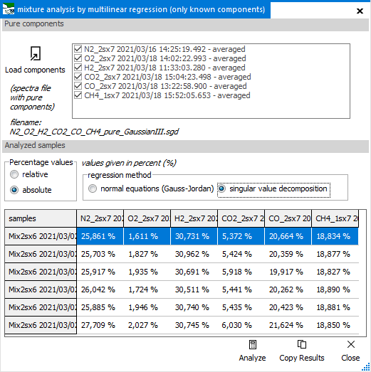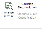
Mixture Analysis This function calculates the amounts of known components in a mixture of unknown composition, based on the given reference spectra for the rpure components. This done by using a multilinear regression algorithm (MLR), which can be used with either normal equations, or singular value decompositon method. With the Load components button, the reference spectra of pure compounds get introduced into the system. You can select or unselect any of them, to devide which will be used in the analysis. The software will remember them, so it can ber used repeatedly. In the data table below, the analysis results for all loaded spectra are shown after clicking the Analyze button. The percentage result can be displayed as relative value, which is the original result, or else as absolute value, which makes all entries sum up to 100%. This is a quite new feature and needs to be thoroughly validated by yourself with known data, before going into the unkown. I found that measurement noise and noisy baselines degrade the results. Therefore I introduced the Gaussian Deconvolution function (described below), which gives a noise-free approximation of a spectrum, ideally suited as input to the MLR algorithm.

<jump back to top>

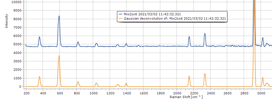
Gaussian Deconvolution This function creates a noise-free spectrum approximation based on Gaussian peaks replacing actual spectrum peaks. This is not (yet) an iterative, fitting algorithm, so "deconvolution" is probably no the right wording. Instead it simply looks for spectrum peaks and creates a Gaussian curve instead, based on peak height and width. It works pretty well on Raman spectra with not too many/ not overlapping peaks and can be used as input for the mixture analysis function (described above). Two alternative ways for peak finding area available: - percentage of max-min: takes a relative lower threshold and combines that with a prominence values (as known from the Peak Labels function) - baseline noise level: caculates the lower threshold from a multiple of the baseline noise in a user-defined area

<jump back to top>

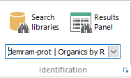
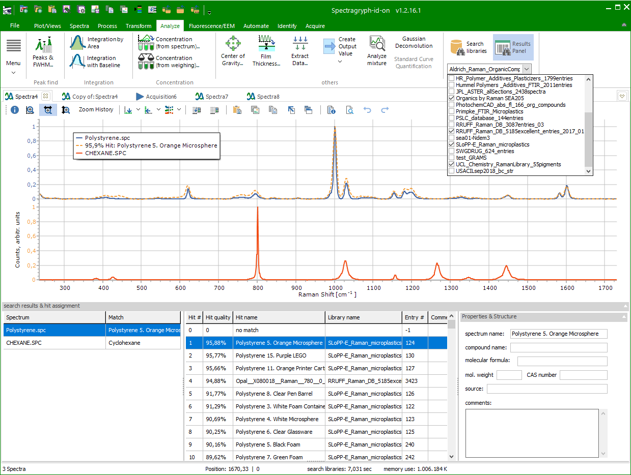
Identification (through spectral library search) This area allows multi-library search for all loaded spectra in an ordinary spectra tab, with display of found hit names and values and library spectra within the plot. First, select the libraries to be searched in the dropdown library selector, which shows the names of all libraries in the libraries folder (usually: C:\Users\Public\Documents\Spectragryph\Libraries\, to be defined in the Identification options ). In options, you can also define the match threshold, and whether to display found reference spectra in the plot and if they should be normalized to the sample spectra. Then, click the Search Libraries button for actual searching, a progress indicator in the lower status bar shows whats going on. When finished, the Results Panel is filed with the search results, and the best hit for the first spectrum is shown in the spectrum plot. The lower results panel shows this interactive content: - the spectra list (at left) with their best hit (or "no match") if no hit above the match threshold was found - the hit list (in the middle) showing the best 20 hits for the selected spectrum, with their hit quality value, spectrum name, library name, and so on - the properties & structure information (at left) for a selected hit, as found in the spectral library Scrolling (left mouse click, mouse wheel or keys) through the hit list will update the displayed reference spectrum above. Clicking on a spectrum or its legend text in the plot, or selcting it in the spectrum list (at left in results panel), will update the plot to show the assigned hit as reference spectrum, with the hit quality as part of the legend text. HINT: the same multi-library search and display of results is also available as post-processing function while acquiring spectra in the Acquire ribbon. Therefore you can have live sample identification during continuous measurement.

<jump back to top>