Spectragryph
- optical spectroscopy software -

Functions of the Transform ribbon => Click onto a button for descriptions

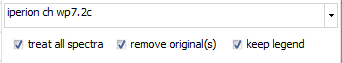
General options: For most functions, you will get a specific window for setting parameters and options. Some options are identical for most of the functions: - At the top, there is a dropdown selector containing the current spectra list. Here you can select the spectrum to be processed (if only one spectrum gets treated). If a preview is available, the spectrum is selected here. - if the "treat all spectra" option is checked, all spectra will get processed and attached as new spectra at the end of the spectrum list. Otherwise, only the currently selected spectrum gets processed. - With the "remove all" option checked, the original spectra will be removed and only the processed spectra/ spectrum remain(s) . - The "keep legend" option leaves the original legend text unchanged. If unchecked, a function-specific text part will be added to the legend text.

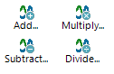
Basic arithmetics Add will add the y values of the two spectra selected in the dropdown lists. If "treat all spectra" is selected, the spectrum selected in the lower list will be added to all spectra. Subtract will subtract the y values of the lower spectrum from the upper spectrum. If "treat all spectra" is selected, the spectrum selected in the lower list will be subtracted from all spectra. Multiply will multiply the y values of the two spectra selected in the dropdown lists. If "treat all spectra" is selected, the spectrum selected in the lower list will be multiplied with all spectra. Divide will divide the y values of the upper spectra from the lower spectrum. If "treat all spectra" is selected, all spectra will get divided by the spectrum selected in the lower list.

<jump back to top>

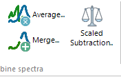
Averaging The y values of the selected spectra (left mouse) will be averaged, using either arithmetic mean or median as calculation method. For selecting spectra to be averaged, some sophisticated options are available for spectra series, based on naming or numbering schemes within the legend texts. The legend text of the averaged spectrum can be entered manually, or derived from one of the used spectra by left-mouse double-clicking its entry. Merging The selected spectra (left mouse) will be merged into a single spectrum, by averaging the overlapping parts with smooth transitions, or interpolating gaps. For selecting spectra to be merged, some sophisticated options are available for spectra series, based on naming schemes within the legend texts, or automated assignment for spectra coming as sub files from a common spectrum file( e.g. from Avantes multi-channel system). The legend text of the merged spectrum can be entered manually, or derived from one of the used spectra by left-mouse double-clicking its entry. 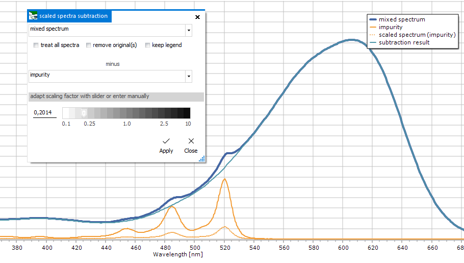Scaled Subtraction For subtracting a spectrum after scaling it with a factor. This factor can be determined interactively by moving the slider or manually entering the scaling factor. During this, the plot will show and live update the scaled spectrum and the subtraction result.

<jump back to top>

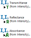
Transmittance & Reflectance (from Intensity) From two intensity spectra (sample and background/ reference), the transmittance or reflectance will be calculated after T = I / I0, resp. R = I / I0 - For transmittance, the reference spectrum needs to be measured from full light source intensity, and the sample spectrum by passing this light through the sample. - For reflectance, the reference spectrum needs to be measured from full light source intensity reflected from a white reflectance standard, and the sample spectrum by measuring this light source reflected from the sample. Absorbance (from Intensity) From two intensity spectra (sample and background/ reference), the absorbance will be calculated after A = -log(T) with T = I / I0 The reference spectrum needs to be measured from full light source intensity, and the sample spectrum by passing this light through the sample.

<jump back to top>

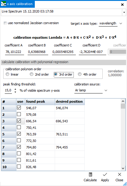X Axis Pixel Calibration For spectra with uncalibrated x axis (pixels), or when you need to recalibrate. Mostly used for measured spectra from controlled spectrometers, therefore also available from the Acquire ribbon. The calibration procedure consists of two steps: 1) calculating the calibration parameters (linear or 2nd to 4th order polynomial), based on a spectrum with known peak positions. Those peak positions get mapped onto the known positions with a polynomial regression. 2) applying the polynomial calibration parameters upon the selected spectrum's x axis values and assigning the new axis type. It is possible to calibrate for - absorbance: by using a sample with known peaks, like a Holmium or Didymium filter. Target: wavelength scale - fluorescence: by using a light source with known emission peaks, like a pen lamp source (Hg, Hg/Ar, Xe, Ne). Target: wavelength scale - Raman shift: by using a sample with known Raman lines, as described in ASTM E1840 standard guide. Target: Raman shift scale For step 1), , open the calibration dialog from the button's dropdown menu. In the upper field, select the spectrum to be used. Change the peak finding threshold, if necessary. Select the desired x axis type after calibration on the right side. Below, the calibration coefficients will be shown, after doing the polynomial regression. In the table below, the x axis positions of the found peaks from the selected spectrum are displayed. You can either enter the known positions into the "desired position" column manually, or select from a number of precompiled positions that are shown as dropdown list. The content of this dropdown list depends on the calibration source chosen above. Only the "custom" option allows to manually enter position values. Check the values to be used during calculation. Finally, select the polynomial order for the regression calculation and press the "Calculate" button. The calculated calibration coefficients will show up in the respective fields above, together withe the regression's correlation coefficient. To keep the coefficients and apply on the selected spectrum (step 2), click the "Apply" button. The peak data for the selectable calibration sources is located in a file called "calibration_lines.csv" in the program folder, this file's content can be changed to adapt or enhance the range of available calibration peak data. The calibration parameters will be remembered for the current session. To make them a permanent setting, go to File > Options > Transform > calibrate x axis For the calibration creating Raman spectra from wavelength spectra, the area-preserving calculation option "use normalized Jacobian conversion" is available. This takes care of the distortion of intensity values caused by the inverse relationship between wavelength and energy, as explained in this publication and its correction. HINT: To better find the peaks to be used during calibration, you might turn on "Peak labels" before starting the calibration procedure.

<jump back to top>

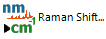
Raman Shift Usually, Raman spectra get measured as wavelength spectra, and are then transformed into Raman spectra, having Raman Shift als x axis type (shown as wavenumbers), calculated after this equation: RamanShift = 10^7/Lambda_exc - 10^7/Lambda The RamanShift is a relative parameter, based on wavelength distance to the actual excitation laser wavelength. therefore, the laser wavelength is always required as input value. It is recommend to use the accurate value, just entering "785" for a 785nm Raman spectrometer wont do the trick, you need the accurate, actual value! Otherwise, you might be several wavenumbers off the truth... As the spectrum's Rayleigh area near the zero point of the Raman Shift scale is often highly distorted, it can be omitted for the transformation, by selecting "cut off Rayleigh peak area" and entering a cutoff value into the "begin Raman spectrum at:" field. For the transformation from wavelength spectra to Raman spectra, the area-preserving calculation option "use normalized Jacobian conversion" is available. This takes care of the distortion of intensity values caused by the inverse relationship between wavelength and energy, as explained in this publication and its correction.

<jump back to top>

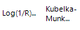
Converting reflectance spectra into "absorbance" Contrary to transmittance spectra, there is no easy way to obtain a corresponding absorbance spectrum from reflectance spectra. Two different methods are available, as explained below. A third one would be based on scattering theory using Kramers-Kronig relations, but this is currently not available in Spectragryph. Log(1/R) method The used equation is already in the name, and looks liike the analogue to caculation fo absorbance from transmittance. The resulting spectra is shown with "log(1/R)" as y unit. This is sometimes used as quick way for creating something absorbance-like, and seems to work best on totally opaque samples. Much discussed on the internet... Kubelka-Munk transformation For the calculation of absorbance from diffuse reflectance spectra, best used on samples with semi-infinite layer thickness, after this equation: k/s = (1-R)^2 / (2*R) The resulting spectra is shown with "Kubelka-Munk units (K/S)" as y unit. For a more detailed treatment of both methods, also refer to the Wiki entries on Kubelka-Munk theory and Diffuse reflectance spectroscopy

<jump back to top>

Derivative The first, second, third or fourth derivative of the spectrum selected in the drop down list will be calculated. The smoothing option is strongly recommended for all derivatives higher than the first derivative. Interpolate, Resample This is the only place to assign a differing x or y axis type to existing data (use with care!). It is also possible to redefine start value, end value and x step width for interpolation to a new set of data points. This can be useful for bringing diverse spectra onto a common scale, before further processing with a chemometric package. Spectrum from Image For the transformation of a spectrum image file into actual spectral data, by converting a horizontal cross-section of a loaded image into intensity data. first load an image file with the "Load image" button (bmp, gif, jpg and png files accepted), then select the actual spectrum area with the ROI rectangle (visible on checking "use spectrum ROI"). For a coarse linear x axis calibration, you can directly set the start and end value in wavenumbers, alternatively the normal x axis calibration is also applicable (see above). The clipping indicator will warn of clipping in any of the colour channels, which means you are loosing linear correlation of actual to measured intesity to some extent.

<jump back to top>